One Dimension

We start by considering the one dimensional Poisson's equation

$$\left.\d^2 V\over\d x^2\right. = f(x).$$ (3.2)

The 2nd derivative may be discretised in the usual way to give

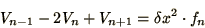$$V_{n-1} - 2 V_n + V_{n+1} = \delta x^2\cdot f_n$$ (3.3)

where we define $f_n = f(x = x_n = n\delta x)$.

The boundary conditions are usually of the form $V(x) = V_0$ at $x = x_0$ and $V(x) = V_{N+1}$ at $x = x_{N+1}$, although sometimes the condition is on the first derivative. Since $V_0$ and $V_{N+1}$ are both known the $n=1$ and $n=N$ equations (3.3) may be written as

$$-2 V_1 + V_2 = \delta x^2\cdot f_1 - V_0$$ (3.4)

$$V_{N-1} - 2 V_N = \delta x^2\cdot f_N - V_{N+1}.$$ (3.5)

This may seem trivial but it maintains the convention that all the terms on the left contain unknowns and everything on the right is known. It also allows us to rewrite the (3.3) in matrix form as

$$\left[\begin{array}{llllllll} -2 &1 & & & & & & \\ 1 &-2 &1... ...ot f_{N-1}\\ \delta x^2\cdot f_N - V_{N+1} \end{array}\right]$$ (3.6)

which is a simple matrix equation of the form

$$\bss{A}\bi{x} = \bi{b}$$ (3.7)

in which $\bss{A}$ is tridiagonal. Such equations can be solved by methods which we shall consider below. For the moment it should suffice to note that the tridiagonal form can be solved particularly efficiently and that functions for this purpose can be found in most libraries of numerical functions.

There are several points which are worthy of note.

• We could only write the equation in this matrix form because the boundary conditions allowed us to eliminate a term from the 1st and last lines.
• Periodic boundary conditions, such as $V(x+L) = V(x)$ can be implemented, but they have the effect of adding a non-zero element to the top right and bottom left of the matrix, $A_{1N}$ and $A_{N1}$, so that the tridiagonal form is lost.
• It is sometimes more efficient to solve Poisson's or Laplace's equation using Fast Fourier Transformation (FFT). Again there are efficient library routines available (Numerical Algorithms Group, n.d.). This is especially true in machines with vector processors.