The Analytical Solution

Next: Choosing an Algorithm Up: A Uniform Field Previous: Units

The Analytical Solution

In order to understand the behaviour of the various methods for ODEs we need to know the analytical solution of the problem. 2 dimensional problems such as this one are often most easily solved by turning the 2D vector into a complex number. Thus by defining $\tilde v = v_x +\i v_y$ we can rewrite (1.43) in the form

$\begin{displaymath} {\d\tilde v\over\d t} = -\i\tilde v\left(qB\over m\right) -\tilde v\left(\gamma\over m\right) \end{displaymath}$

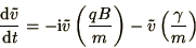(1.48)

which can be easily solved using the integrating factor method to give

$\begin{displaymath} \tilde v = \tilde v_0 \exp\left[-\i\left(qB\over m\right)t -\left(\gamma\over m\right)t\right]. \end{displaymath}$

(1.49)

Finally we take real and imaginary parts to find the

and

components

$\displaystyle v_x$	$\textstyle =$	$\displaystyle +v_0\cos\left[\left(qB\over m\right)t + \phi_0\right] \exp\left[-\left(\gamma\over m\right)t\right]$	(1.50)
$\displaystyle v_y$	$\textstyle =$	$\displaystyle -v_0\sin\left[\left(qB\over m\right)t + \phi_0\right] \exp\left[-\left(\gamma\over m\right)t\right]$	(1.51)