Next: Oscillating Electric Field
Up: Project Classical
Previous: Choosing an Algorithm
Crossed Electric and Magnetic Fields
You are now in a position to apply your chosen algorithm to a more
complicated
problem. In addition to the uniform magnetic field,  , we now
add an electric field in the
, we now
add an electric field in the  -direction,
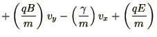
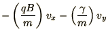
 . Thus (1.43a) must be modified
to read
. Thus (1.43a) must be modified
to read
You should now write a program to solve (1.9.2) using the most
appropriate method as found
earlier.
Try to investigate the behaviour of the system in various physical
regimes. You should also vary  to check whether the stability
conforms to your expectations.
Think about the physical system you are describing and whether your
results are consistent with the behaviour you would expect.
to check whether the stability
conforms to your expectations.
Think about the physical system you are describing and whether your
results are consistent with the behaviour you would expect.