


Next: Euler Method
Up: Ordinary Differential Equations
Previous: Ordinary Differential Equations
In this chapter we will consider the methods of solution of the sorts of
ordinary differential equations (ODEs) which occur very commonly in
physics. By ODEs we mean equations involving derivatives with respect to
a single variable, usually time. Although we will formulate the
discussion in terms of linear ODEs for which we know the analytical
solution, this is simply to enable us to make comparisons between the
numerical and analytical solutions and does not imply any restriction on
the sorts of problems to which the methods can be applied. In the
practical work you will encounter examples which do not fit neatly into
these categories.
The work in this section is also considered in chapter 16
of Press et al. (1992) or chapter II of
Potter (1973)
We consider 3 basic differential equations:
which are representative of most more complex cases.
Higher order differential equations can be reduced to 1st order
by appropriate choice of additional variables. The simplest such choice
is to define new variables to represent all but the highest order
derivative. For example, the damped
harmonic oscillator equation, usually written as
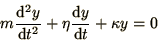 |
(1.4) |
can be rewritten in terms of  and velocity
  in the form
of a pair of 1st order ODEs
in the form
of a pair of 1st order ODEs
Similarly any  th order differential equation can be reduced to
1st order equations.
Such systems of ODEs can be written in a very concise notation by
defining a vector,
th order differential equation can be reduced to
1st order equations.
Such systems of ODEs can be written in a very concise notation by
defining a vector,  say, whose elements are the unknowns, such as
and
say, whose elements are the unknowns, such as
and  in (1.1). Any ODE in unknowns can then be
written in the general form
in (1.1). Any ODE in unknowns can then be
written in the general form
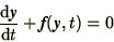 |
(1.7) |
where and  are -component vectors.
Remember that there is no significance in the use of the letter
are -component vectors.
Remember that there is no significance in the use of the letter  in
the above equations. The variable is not necessarily time but could
just as easily be space, as in (1.9), or some other physical
quantity.
Formally we can write the solution of
(1.7) as
in
the above equations. The variable is not necessarily time but could
just as easily be space, as in (1.9), or some other physical
quantity.
Formally we can write the solution of
(1.7) as
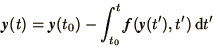 |
(1.8) |
by integrating both sides over the interval
 .
Although (1.8) is formally correct, in practice it is
usually impossible to evaluate the integral on the right-hand-side as
it presupposes the solution
.
Although (1.8) is formally correct, in practice it is
usually impossible to evaluate the integral on the right-hand-side as
it presupposes the solution  . We will have to employ an
approximation.
All differential equations require boundary conditions. Here we will
consider cases in which all the boundary conditions are defined at a
particular value of (e.g.
. We will have to employ an
approximation.
All differential equations require boundary conditions. Here we will
consider cases in which all the boundary conditions are defined at a
particular value of (e.g.  ). For higher order equations the
boundary conditions may be defined at different values of .
The modes of a violin string at frequency
). For higher order equations the
boundary conditions may be defined at different values of .
The modes of a violin string at frequency  obey the equation
 |
(1.9) |
with boundary conditions such that  at both ends of the string. We
shall consider such problems later.
at both ends of the string. We
shall consider such problems later.
Next: Euler Method
Up: Ordinary Differential Equations
Previous: Ordinary Differential Equations


