A Simple Method

We consider the diffusion equation and apply the same simple method we tried for the hyperbolic case.

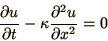$${\partial u\over\partial t} - \kappa{\partial^2 u\over\partial x^2} = 0$$ (2.26)

and discretise it using the Euler method for the time derivative and the simplest centred 2nd order derivative to obtain

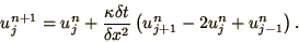$$u_j^{n+1} = u_j^n + {\kappa\delta t\over\delta x^2} \left(u_{j+1}^n - 2 u_j^n + u_{j-1}^n\right).$$ (2.27)

Applying the von Neumann analysis to this system by considering a single Fourier mode in $x$ space, we obtain

$$v^{n+1} = v^n\left[ 1 - {4\kappa\delta t\over\delta x^2}\sin^2\left(k\delta x\over 2\right) \right]$$ (2.28)

so that the condition that the method is stable for all $k$ gives

$$\delta t \le {\mathchoice{{\textstyle{\frac12}}}{{\textstyl... ...le{1/2}}}{{\scriptscriptstyle{1/2}}}}{\delta x^2\over\kappa}.$$ (2.29)

Although the method is in fact conditionally stable the condition (2.29) hides an uncomfortable property: namely, that if we want to improve accuracy and allow for smaller wavelengths by halving $\delta x$ we must divide $\delta t$ by $4$. Hence, the number of space steps is doubled and the number of time steps is quadrupled: the time required is multiplied by $8$. Note that this is different from the sorts of conditions we have encountered up to now, in that it doesn't depend on any real physical time scale of the problem.