Schrödinger's equation

In dimensionless form the time-independent Schrödinger equation can be written as

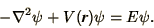$$-\nabla^2\psi + V(\bi{r})\psi = E\psi.$$ (3.16)

The Laplacian, $\nabla^2$, can be represented in discrete form as in the case of Laplace's or Poisson's equations. For example, in 1D (3.16) becomes

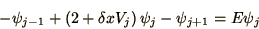$$-\psi_{j-1} + \left(2 + \delta x V_j\right)\psi_j - \psi_{j+1} = E\psi_j$$ (3.17)

which can in turn be written in terms of a tridiagonal matrix $\bss{H}$ as

$$\bss{H}\underline{\psi} = E\underline{\psi}.$$ (3.18)

An alternative and more common procedure is to represent the eigenfunction in terms of a linear combination of basis functions so that we have

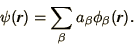$$\psi(\bi{r}) = \sum_\beta a_\beta \phi_\beta(\bi{r}).$$ (3.19)

The basis functions are usually chosen for convenience and as some approximate analytical solution of the problem. Thus in chemistry it is common to choose the $\phi_\beta$ to be known atomic orbitals. In solid state physics often plane waves are chosen. Inserting (3.19) into (3.16) gives

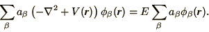$$\sum_\beta a_\beta \left(-\nabla^2 + V(\bi{r})\right)\phi_\beta(\bi{r}) = E \sum_\beta a_\beta \phi_\beta(\bi{r}).$$ (3.20)

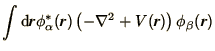
Multiplying this by one of the $\phi$'s and integrating gives

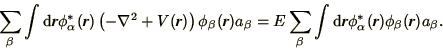$$\sum_\beta \int\d\bi{r} \phi^*_\alpha(\bi{r}) \left(-\nabl... ...\int\d\bi{r}\phi^*_\alpha(\bi{r})\phi_\beta(\bi{r}) a_\beta.$$ (3.21)

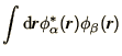
We now define 2 matrices

$$\bss{H}\equiv H_{\alpha\beta} = \int\d\bi{r} \phi^*_\alpha(\bi{r}) \left(-\nabla^2 + V(\bi{r})\right)\phi_\beta(\bi{r})$$ (3.22)

$$\bss{S}\equiv S_{\alpha\beta} = \int\d\bi{r}\phi^*_\alpha(\bi{r})\phi_\beta(\bi{r})$$ (3.23)

so that the whole problem can be written concisely as

$$\sum_\beta H_{\alpha\beta}a_\beta = E \sum_\beta S_{\alpha\beta} a_\beta$$ (3.24)

$$\bss{H}\bi{a} = E \bss{S}\bi{a}$$ (3.25)

which has the form of the generalised eigenvalue problem. Often the $\phi$'s are chosen to be orthogonal so that $S_{\alpha\beta} = \delta_{\alpha\beta}$ and the matrix $\bss{S}$ is eliminated from the problem.