


Next: The Leap-Frog Method
Up: Euler Method
Previous: Application to Non-Linear Differential
A little more care is required when  and
and  are vectors.
In this case
are vectors.
In this case  is an arbitrary infinitesimal vector and the
derivative
is an arbitrary infinitesimal vector and the
derivative
 is a matrix
  with
components
with
components
 |
(1.25) |
in which  and
and  represent the components of and
respectively. Hence (1.18) takes the form
represent the components of and
respectively. Hence (1.18) takes the form
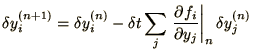 |
|
|
(1.26) |
![$\displaystyle \delta\bi{y}_{n+1} =\left[\bss{I} - \delta t \bss{F}\right]\delta\bi{y}_n= \bss{G}\delta\bi{y}_n.$](img77.png) |
|
|
(1.27) |
This leads directly to the stability condition that all the eigenvalues
of  must have modulus less than unity (see
problem 6).
In general any of the stability conditions derived in this course for scalar
equations can be re-expressed in a form suitable for vector equations
by applying it to all the eigenvalues of an appropriate matrix.
must have modulus less than unity (see
problem 6).
In general any of the stability conditions derived in this course for scalar
equations can be re-expressed in a form suitable for vector equations
by applying it to all the eigenvalues of an appropriate matrix.