Next: The Runge-Kutta Method
Up: Ordinary Differential Equations
Previous: Application to Vector Equations
The Leap-Frog Method
How can we improve on the Euler method? The most obvious way would be to
replace the forward difference in (1.12) with a
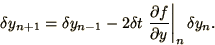
centred difference (1.13) to get the formula
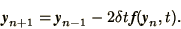 |
(1.28) |
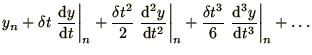
If we expand both  and
and  as
before
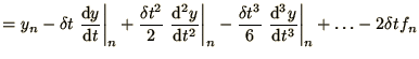
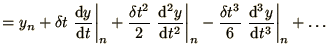
(1.28) becomes
as
before
(1.28) becomes
from which all terms up to  cancel so that the method
is clearly 2nd order accurate.
Note in passing that using (1.28) 2 consecutive values of
cancel so that the method
is clearly 2nd order accurate.
Note in passing that using (1.28) 2 consecutive values of
 are required in order to calculate the next one: and
  are required to calculate
  . Hence 2 boundary conditions
are required, even though (1.28) was derived from
a 1st order differential equation.
This so-called leap-frog method is more accurate than
the Euler method, but is it stable? Repeating the
same analysis
as for the Euler method we again obtain a linear equation
for
. Hence 2 boundary conditions
are required, even though (1.28) was derived from
a 1st order differential equation.
This so-called leap-frog method is more accurate than
the Euler method, but is it stable? Repeating the
same analysis
as for the Euler method we again obtain a linear equation
for 
 |
(1.31) |
We analyse this equation by writing
 and
and
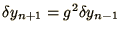 to obtain
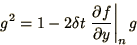 |
(1.32) |
which has the solutions
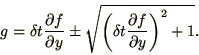 |
(1.33) |
The product of the 2 solutions is equal to the constant in the quadratic
equation, i.e.  . Since the 2 solutions are different, one of them
always has magnitude
. Since the 2 solutions are different, one of them
always has magnitude  . Since for a small random error it is
impossible to guarantee that there will be no contribution with
. Since for a small random error it is
impossible to guarantee that there will be no contribution with  this contribution will tend to dominate as the equation is iterated.
Hence the method is unstable.
There is an important exception to this instability: when the partial
derivative is purely imaginary (but not when it has some general complex
value), the quantity under the square root in (1.33) can be
negative and both
this contribution will tend to dominate as the equation is iterated.
Hence the method is unstable.
There is an important exception to this instability: when the partial
derivative is purely imaginary (but not when it has some general complex
value), the quantity under the square root in (1.33) can be
negative and both  's have modulus unity. Hence, for the case of
oscillation (1.1c) where
's have modulus unity. Hence, for the case of
oscillation (1.1c) where
 , the algorithm is just stable, as long as
 |
(1.34) |
The stability properties of the leap-frog method are summarised below
| Decay |
Growth |
Oscillation |
| unstable |
unstable |
 |
Again the growth equation should be analysed somewhat differently.
Next: The Runge-Kutta Method
Up: Ordinary Differential Equations
Previous: Application to Vector Equations